We’ve covered IP in depth; how packets are structured, addressed, and handed off between layers. We went through TCP’s reliability and UDP’s lean, no-guarantee model.
But there’s a gap we left open.
We kept saying “packets hop through routers” without ever explaining how a router actually decides where to send something.
The internet spans billions of devices across hundreds of thousands of independent networks, and yet a packet sent from Tokyo can find its way to a server in Podgorica in under 200 milliseconds. Something has to be making very fast, very accurate decisions at every step of that journey.
That something is IP routing.
Every router along a packet’s path maintains a table of known networks and makes a forwarding decision in milliseconds; sometimes in hardware, at line speed.
These decisions are informed by routing protocols running continuously in the background, letting routers share information, react to failures, and converge on the best available path.
That’s what we’re opening up today.
Foundation
Before we get into how routing works, we need to make sure a few concepts are solid. Nothing new here if you’ve been following along, just tightening the foundation before we build on it.
IP Addresses and Networks
Every device on the internet has an IP address. You can think of it like a postal address, it tells the network where something lives.
But addresses don’t exist in isolation. They’re grouped into networks, and those groups are defined by a subnet mask.
So basically an IP address identifies a device on a network, while a subnet mask determines which part of that IP refers to the network and which part refers to the specific device (host) within that network.
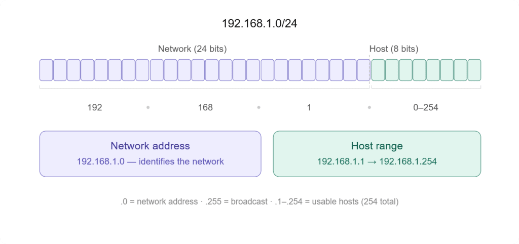
Take 192.168.1.0/24 the /24 means the first 24 bits identify the network, and the remaining 8 bits identify individual devices within it. Everything in that range, from 192.168.1.1 to 192.168.1.254, lives on the same network.
Why does this matter? Because a router’s entire job depends on it. When a packet arrives, the router looks at the destination IP and asks: which network does this belong to? That question is what drives every forwarding decision.
Hosts vs Routers
A host is any device that sends or receives data: your laptop, a server, a phone. It has an IP address, it generates traffic, but it doesn’t make routing decisions.
If a host needs to send something outside its own network, it just hands it off to a router and forgets about it.
The router sits between networks and its entire purpose is to move packets from one network toward another. It has multiple interfaces, each connected to a different network, and it makes deliberate decisions about where each packet goes next.
The line matters because routing logic lives in routers, not hosts.
Hopping
Every time a packet moves from one router to the next, that’s a hop. A packet traveling across the internet doesn’t go directly from source to destination, it passes through a series of routers, each one getting it a little closer.
Each hop is a separate forwarding decision made by a separate router. By the time a packet reaches its destination it may have crossed dozens of them.
The Default Gateway
When a host wants to send traffic outside its own network, it needs somewhere to send it. That somewhere is the default gateway, usually the router sitting at the edge of the local network.
The host doesn’t know the full path to the destination. It doesn’t need to. It just hands the packet to the gateway and lets the routing infrastructure figure out the rest.
This is the handoff point where routing actually begins.
The Routing Table
Every router has a routing table. It’s the core data structure that makes forwarding decisions possible, a list of known networks and instructions for how to reach them.
When a packet arrives, the router doesn’t guess. It looks up the destination IP in this table and follows what it finds.
Let’s see what a routing table looks like.
Destination       Gateway         Genmask         Iface   Metric
192.168.1.0       0.0.0.0         255.255.255.0   eth0    0
10.0.0.0          10.0.0.1        255.0.0.0       eth1    10
0.0.0.0 192.168.1.1 0.0.0.0 eth0 0The destination is the network the router knows about.
The gateway is where to forward the packet next: 0.0.0.0 means the destination is directly reachable on that interface without going through another router.
Genmask is the subnet mask that determines which IP addresses belong to a specific network when routing traffic.
The interface is which physical or virtual port to send it out of. The metric is the cost, lower is preferred when multiple paths exist.
A physical port is a hardware interface on a device where cables connect, while a virtual port is a logical communication endpoint used by software to manage network traffic.
Genmask
Now let’s pick a row and deepen our understanding of the Genmask (subnet mask).
Destination       Gateway         Genmask         Iface   Metric
10.0.0.0 10.0.0.1 255.0.0.0 eth1 10An IPv4 address like x.x.x.x has four parts called octets. Each octet is 8 bits. IP addresses are written in decimal, but each number represents 8 binary bits, meaning each value ranges from 0 to 255. So an IPv4 address is 32 bits in total (4 × 8 bits).
If a network uses a /16 prefix, it means the first 16 bits (the first two octets) define the network part, and the remaining 16 bits are used for hosts (devices). For example, 192.168.0.0/16 means all addresses from 192.168.0.0 to 192.168.255.255 are in the same network.
If “defining a network” sounds too fancy, just think of it as each network is just a random number, 10 could just be 2. We are simply using it to create different networks for devices.
In this case, you can have up to 65,534 usable host addresses. That’s because 16 bits for hosts gives 2¹⁶ total addresses.
255.0.0.0 means /8, so if you want to reach 10.0.0.1 (or any 10.x.x.x address), your machine sends the packet to the next-hop gateway listed in the route, which is 10.0.0.1.
If you want to see how to convert 255.0.0.0 to CIDR (/8) in detail, it works like this:
255   = 11111111
0     = 00000000
0     = 00000000
0     = 00000000

Full mask:
11111111.00000000.00000000.00000000

Count 1 bits:
8

Final:
255.0.0.0 = /8
For more information about bits, bytes, and octets, you might want to check this article.
Prefix Match
When a packet arrives, the router compares the destination IP against every entry in the table.
If multiple entries match, the most specific one wins; the one with the longest prefix, meaning the most bits locked down.
If you ask why, when multiple routes match an IP, the router picks the most specific (longest prefix) because it represents a smaller, more precise network.
A smaller, more specific network reduces ambiguity. The router can more accurately decide where the packet should go, instead of using a broad general route.
Say the table has these two entries:
10.0.0.0/8     → via eth0
10.1.0.0/16 → via eth1A packet destined for 10.1.5.3 matches both. But /16 is more specific than /8, so it goes out eth1.
This is longest prefix match and it’s the fundamental rule every router follows.
The Default Route
That third entry in the example above, 0.0.0.0/0, is the default route. It matches everything, but it’s the least specific entry possible.
Any packet that doesn’t match a more specific entry falls through to this.
It’s the router’s way of saying: I don’t know exactly where this goes, but send it here and let someone else figure it out.
For most edge routers, this points toward the ISP.
Without a default route, any packet destined for an unknown network gets dropped.
Administrative Distance
Routing tables can be populated by multiple sources, you might have a static route and OSPF both claiming to know how to reach the same network. The router needs a tiebreaker.
Don’t worry, OSPF, static routes, and everything else will be explained later.
That tiebreaker is administrative distance, a number that ranks the trustworthiness of the source. Lower is more trusted.
| Source | Type of Route | Administrative Distance |
|---|---|---|
| Directly connected | Directly connected | 0 |
| Static route | Static route | 1 |
| RIP | Dynamic routing protocol | 120 |
| OSPF | Dynamic routing protocol | 110 |
If a directly connected route and an OSPF route both point to the same destination, the directly connected one wins.
It’s not about speed, it’s about how much the router trusts the source of that information.
Building Routing Table
To build a routing table, there are three sources of routes: directly connected routes, static routes, and dynamic routing protocols.
Directly connected routes are automatic. The moment you assign an IP to an interface and bring it up, the router adds that network to the table. No configuration needed.
Static routes are manual. You tell the router: to reach this network, send traffic here. Simple but doesn’t adapt if something breaks.
Dynamic routing protocols are automatic and adaptive. Routers running the same protocol exchange information with each other, building a picture of the wider network.
When something changes, a link goes down, a new network appears, the table updates. This is how large networks stay operational without someone manually updating every router.
We’ll go deep on the protocols in the next chapter. For now, the key point is that the routing table is the product of all three sources combined, with administrative distance deciding what gets used when they conflict.
Initializing a Routing Table
We’ve talked about the sources used to build a routing table, now it’s time to broaden the topic, because this isn’t something that can be properly explained in a simple subheader.
A routing table isn’t something that just “exists” on a router. It is built and continuously updated using different sources of routing information. Every entry in that table answers a simple question:
To reach this destination network, where should I send the packet next?
Routers populate routing tables through three main mechanisms: directly connected networks, static configuration, and dynamic routing protocols (which themselves include multiple categories).
Directly Connected Networks
This is the most basic and automatic way a router learns routes.
When you configure an IP address on an interface and bring it up, the router immediately installs a route for that network in its routing table. No extra configuration.
So if an interface is configured as 192.168.1.1/24, the router automatically understands:
I can reach 192.168.1.0/24 directly through this interface.
Think of interfaces as “portals” that connect your device (host) to other devices or the internet. These can include Ethernet ports (wired), Wi-Fi adapters (wireless), and virtual interfaces (used for VPNs, Docker, etc.). These are all different types of network interfaces.
There are network interfaces such as eth0, eth1, and wlan0.
eth0 is simply a name for a network interface and is traditionally used for Ethernet (wired) connections. It is not specifically tied to a particular network or location. For example, eth0 could be connected to your office network, while eth1 could be connected to another network, such as at home. There is no fixed rule for what each interface must represent; the names are just labels assigned by the system.
You can also connect a single network using two different interfaces, though you’d probably only do that if you enjoy making your routing table slightly more dramatic for no reason.
Wi-Fi interfaces are usually named wlan or newer names like wlp…. These are specifically used for wireless connections, even though the data is ultimately transmitted over Ethernet-like frames internally.
Other common interfaces include lo for loopback (internal communication within your own device), tun or tap for VPN tunnels, and br for network bridges.
Back to the topic, directly connected network routes form the foundation of the routing table. All other routes depend on them.
Static Routes
Static routes are the manual layer.
Here, an administrator explicitly tells the router how to reach a specific network by defining a next hop or an exit interface.
It’s basically: “If you want to reach this network, go that way.”
Static routing is simple and predictable. It’s useful for small, stable networks, default routes toward an ISP, and simple branch or edge setups.
But in complex networks, you typically avoid it, it becomes a nightmare to configure and debug at scale.
Dynamic Routing Protocols
Instead of manually defining routes, routers use dynamic routing protocols to talk to each other and learn the network automatically. They share information, calculate the best paths, and update the routing table whenever something changes.
This is what makes large networks actually possible to run.
Dynamic routing protocols generally fall into three categories: Distance Vector, Link State, and Path Vector. They all solve the same problem, how to reach a destination, but in very different ways depending on scale and complexity.
Dynamic Routing Protocols
This chapter will explain the three routing algorithms in detail: Distance Vector, Link State, and Path Vector.
Distance Vector Routing
Distance vector protocols are the simplest form of dynamic routing.
The idea is straightforward: “I don’t need to know the full network. I just need to know what my neighbor knows.”
Routers using distance vector protocols periodically share their routing tables with directly connected neighbors. They don’t build a full map of the network. Instead, they rely on second-hand information that slowly propagates through the network.
Each route is evaluated based on a metric, such as hop count, bandwidth, or delay, depending on the protocol.
RIP (Routing Information Protocol)
RIP is the classic example of distance vector routing. It uses hop count as its only metric, with a maximum of 15 hops (16 is considered unreachable).
Because of its simplicity, RIP works in very small networks, but it doesn’t scale well in complex environments.
RIP relies on hop count to make routing decisions. A hop count of 0 means the network is directly connected, 1 hop means one router away, and so on. Based on this, it determines where to send traffic next.
EIGRP (Enhanced Interior Gateway Routing Protocol)
EIGRP (Enhanced Interior Gateway Routing Protocol) is a more advanced example of distance vector routing.
Unlike RIP, it uses a composite metric that takes into account bandwidth, delay, reliability, and load to calculate the best path.
It is simple to configure, but much more efficient and scalable than RIP.
Because of its improved design, EIGRP works well in medium to large networks and converges much faster when the network changes.
Instead of relying only on hop count, EIGRP evaluates multiple factors to determine the best route. This allows it to choose more optimal paths and avoid inefficient routing decisions.
Think of it like RIP with extra steps.
Link State Routing
Link state takes a completely different approach.
Instead of blindly trusting neighbors, each router builds a full map of the network.
The idea is: “Everyone shares their links. I build the full picture myself.”
Routers flood information about their directly connected links to all other routers in the network (or area). This information is stored in a database called the LSDB (Link State Database).
Once every router has the same map, each one independently calculates the best path using an algorithm called SPF (Shortest Path First).
OSPF (Open Shortest Path First)
OSPF is one of the most widely used link-state routing protocols. It is designed for enterprise networks and focuses on fast convergence and efficient routing.
It works by building a complete map of the network inside an area. Each router floods information about its directly connected links, and all routers store this data in the LSDB (Link State Database).
Once the LSDB is built, OSPF uses the SPF (Shortest Path First) algorithm to calculate the best path to every destination.
OSPF organizes networks into areas to improve scalability. This reduces overhead and limits how much routing information each router needs to process.
Because of this design, OSPF is fast, scalable, and very stable in large internal networks.
The tradeoff is complexity and resource usage, maintaining the database and running SPF calculations takes CPU and memory.
IS-IS (Intermediate System to Intermediate System)
IS-IS is another link-state routing protocol, very similar in concept to OSPF but often used in service provider and large backbone networks.
Like OSPF, IS-IS builds a full topology map by flooding link-state information and storing it in a database. Each router then independently calculates the best path using SPF.
The key difference is in its design structure. IS-IS is more flexible and simpler in its hierarchy compared to OSPF, which uses areas in a more rigid way.
Because of this, IS-IS scales extremely well and is often preferred in very large networks like ISP backbones.
Path Vector (BGP)
Path vector routing is completely different from both distance vector and link state. It is designed for one specific purpose: routing between different networks on the internet.
Distance vector and link-state protocols are used for internal routing within a network, while path vector routing is used for external routing between different networks across the internet.
Reason
Distance-vector and link-state routing protocols are not used for routing across the global internet because they are designed for intra-domain routing (within a single autonomous system) and do not scale well for inter-domain use.
Distance-vector protocols, such as RIP, have inherent limitations like a maximum hop count (typically 15), slow convergence, and vulnerability to routing loops, which make them unsuitable for large, highly dynamic networks.
Link-state protocols, such as OSPF and IS-IS, while more efficient and accurate, require each router to maintain a complete topology database and perform computationally intensive shortest-path calculations, which increases memory and CPU overhead as the network grows.
In contrast, internet-wide routing between autonomous systems requires not only scalability but also policy-based routing, where different organizations can control how traffic enters, leaves, and traverses their networks based on economic, security, and administrative preferences.
Because distance-vector and link-state protocols lack this level of policy control and do not operate effectively across independently managed networks, the internet uses a different approach: path-vector routing (BGP), which is designed specifically for scalable inter-domain routing with support for policy decisions and control over advertised paths.
Protocol
BGP uses a different approach to routing. Instead of relying on simple metrics like hop count (as in distance-vector protocols) or building a complete network topology map (as in link-state protocols), BGP uses a path-vector mechanism. It records the sequence of autonomous systems a route has passed through (the AS-path) and applies policy-based rules to determine whether a route should be accepted, preferred, or rejected.
Each route carries something called an AS Path, which is basically a list of Autonomous Systems the route has passed through. This helps prevent loops and also gives context about how the route reached you.
BGP doesn’t choose the shortest path. It chooses the most preferred path based on policy.
Routes are selected based on attributes such as AS path length, local policy rules, and network preferences set by administrators.
This makes BGP extremely flexible and highly scalable, but also slower to converge compared to internal routing protocols.
BGP is not trying to find the fastest route, it’s trying to find the allowed route.
That’s why it powers the internet itself, where business rules matter just as much as technical efficiency.
The Forwarding Process
So far, we’ve focused on how routes are learned and stored in a routing table. But there’s another side to the story that often gets confused with routing itself: what actually happens when a packet is sent through the router.
This is where forwarding comes in.
Routing decides where traffic should go. Forwarding is the actual act of moving that traffic.
Routing vs Forwarding
Routing is the decision-making process. It builds the routing table and figures out the best path to every destination using directly connected routes, static routes, and dynamic routing protocols.
Forwarding is the execution process. It takes a packet, looks up the destination, and sends it out of the correct interface.
Control Plane vs Data Plane
Routers are split into two logical planes: the control plane and the data plane.
The control plane is where routing decisions are made. It is responsible for running routing protocols such as OSPF, BGP, and RIP, building and maintaining the routing table (RIB), and learning and updating network topology. In simple terms, it acts as the brain of the router.
The data plane is where actual packet movement happens. It is responsible for forwarding packets based on lookup results, moving traffic from ingress to egress interfaces, and operating at very high speed. In simple terms, it acts as the hands of the router.
RIB & FIB
Inside the router, there are two important tables that separate decision-making from forwarding: the Routing Information Base (RIB) and the Forwarding Information Base (FIB).
The RIB is the full routing table. It is built by the control plane and contains all known routes, including metrics, next-hop information, and best path selection results. It is rich in detail but not optimized for fast forwarding.
The FIB is a simplified, optimized version of the routing table used for actual packet forwarding. It contains only the best routes, next-hop information, and outgoing interface mappings. The FIB is designed for speed, not complexity.
Hardware Forwarding
Modern routers don’t rely only on CPUs to forward packets. That would be too slow for high-speed networks.
Instead, they use hardware acceleration where ASICs (Application-Specific Integrated Circuits) handle forwarding decisions at wire speed, and CAM (Content Addressable Memory) enables extremely fast lookups.
This allows packets to be forwarded in hardware in microseconds without involving the CPU for every packet. This is why modern routers can handle massive traffic loads without breaking down.
Process Switching vs Fast Switching vs CEF
Over time, packet forwarding has evolved in how efficiently it is handled, especially in Cisco environments where different switching methods were introduced.
Process switching is the oldest and slowest method. In this approach, every packet is processed by the CPU, and a routing table lookup happens for each packet individually, making it extremely inefficient for large traffic loads.
Fast switching is an improvement over process switching. In this method, the first packet is processed by the CPU, and the result is cached so that subsequent packets can use the cached entry instead of repeating the lookup process. While better, it is still limited in scalability.
CEF (Cisco Express Forwarding) is the modern standard. It pre-builds the FIB and adjacency table, uses hardware-based lookups when possible, and eliminates per-packet CPU processing. This allows routers to forward traffic at very high speeds with minimal CPU load.
So basically, they use specialized hardware to handle packet forwarding decisions and free up the CPU from processing every packet.
TTL and Loop Prevention
Once packets start moving through routers, one of the biggest problems that can happen is routing loops. A packet can get stuck circulating between routers indefinitely if something goes wrong in the routing logic.
To prevent this, networks use a combination of TTL-based control and routing protocol mechanisms.
How TTL Works
TTL (Time To Live) is a field inside the IP header that acts like a “lifetime counter” for a packet.
Every time a packet passes through a router (each hop), the TTL value is decreased by 1. When the TTL reaches 0, the packet is dropped immediately.
So instead of a packet looping forever, it has a hard limit on how far it can travel. This prevents infinite loops at the IP layer, even if routing is misconfigured.
ICMP Time Exceeded Message
When a packet is dropped because TTL reaches zero, the router doesn’t just silently discard it. It sends back an ICMP Time Exceeded message to the source.
This message tells the sender: Your packet was dropped because it exceeded its TTL limit.
This mechanism is also what tools like traceroute rely on. By intentionally manipulating TTL values, traceroute maps the path a packet takes through the network.
Other Loop Prevention Mechanisms
While TTL protects the network at the packet level, routing protocols also include their own loop prevention mechanisms at the routing level.
Split horizon prevents a router from advertising a route back out of the same interface it was learned from. It’s like saying don’t tell me about a route I already told you.
This reduces the chance of routing loops forming in distance vector protocols.
Route poisoning is a method where a failed or invalid route is advertised with an infinite metric (or a value that represents “unreachable”).
This ensures that all routers in the network quickly learn that the route is no longer valid, instead of continuing to use outdated information.
It basically forces the network to converge faster after a failure.
Hold-down timers introduce a waiting period after a route is marked as down before accepting new updates for that route.
This prevents unstable or incorrect routing information from being immediately reinstalled, especially during network flapping. It’s like waiting before trusting that this route is back.
IPv6 Routing
IPv6 routing is not a completely new concept, it still relies on the same core ideas we’ve already covered: routing tables, dynamic routing protocols, and forwarding decisions.
But the way networks operate changes because IPv6 itself introduces a different design philosophy compared to IPv4.
What Changes in IPv6
The most obvious change is address size. IPv6 uses 128-bit addresses, which massively expands the address space compared to IPv4. This removes the need for techniques like NAT in most cases and allows for more hierarchical network design.
NAT is a mechanism that allows multiple devices on a private network to share a single public IP address.
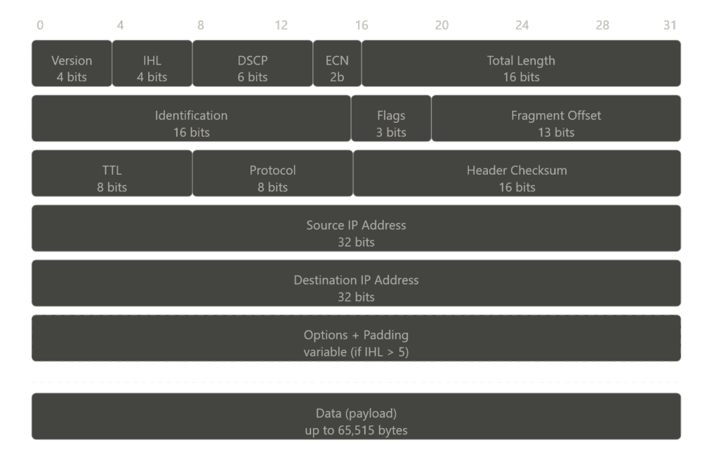
The IPv6 header is also simplified. Unlike IPv4, it removes unnecessary fields and moves optional information into extension headers. This makes packet processing more efficient for routers.
In IPv6, the header checksum, header length, fragmentation fields (ID, flags, fragment offset), and options are removed, while flow label, traffic class, hop limit, and extension headers are added.
Another major change is that IPv6 does not use broadcast. Instead, it relies on multicast and anycast communication. This reduces unnecessary network noise and improves efficiency, especially in large networks.
OSPFv3 and BGP with IPv6
Routing protocols had to evolve to support IPv6, but their core logic remains the same.
OSPFv3
OSPFv3 is the version of OSPF designed for IPv6. It still uses link-state principles, flooding LSAs and building a full topology map, but it operates independently of IPv4 and supports IPv6 prefixes.
BGP with IPv6 (AFI/SAFI)
BGP supports IPv6 using address families (AFI/SAFI). This allows BGP to carry both IPv4 and IPv6 routes within the same protocol framework. The path vector concept remains the same, routing decisions are still based on policy and AS path information.
Dual-Stack and Transition Mechanisms
Since IPv4 and IPv6 will coexist for a long time, transition mechanisms are essential.
Dual-Stack
Dual-stack means a device runs both IPv4 and IPv6 simultaneously. It can communicate using either protocol depending on the destination.
Tunneling
Tunneling allows IPv6 packets to be encapsulated inside IPv4 packets so they can travel across IPv4-only networks.
Translation (NAT64)
Translation mechanisms convert IPv6 traffic to IPv4 and vice versa, allowing communication between different protocol versions.
Routing in Modern Contexts
Routing today is no longer limited to traditional routers and static network diagrams.
Modern networks have become abstracted, virtualized, and distributed across cloud platforms, data centers, and container environments.
While the core principles of routing still apply, the way routing is implemented has evolved significantly.
Software-Defined Networking (SDN)
Software-Defined Networking (SDN) takes the idea of separating the control plane and data plane and extends it to a much larger scale.
Instead of each device making independent routing decisions, SDN centralizes the control logic in a controller.
This controller has a global view of the entire network and programs forwarding rules directly into devices. In simple terms, traditional networking means each router thinks for itself, while SDN means one central brain controls everything.
This approach makes networks more programmable, easier to manage, and highly scalable, especially in large data centers.
Routing in Cloud Environments
In cloud platforms like AWS and GCP, routing is no longer tied to physical routers.
Instead, it is implemented virtually using software-defined constructs. For example, in an AWS VPC, route tables define how traffic flows between subnets, internet gateways, and NAT gateways, behaving like traditional routing tables but fully managed in software.
Cloud environments still use routers, but you don’t interact with them directly. Instead of configuring physical or virtual routers yourself, you work with abstracted components like route tables and networking policies.
The actual routing is handled behind the scenes by the cloud provider using software-defined networking (SDN), where control logic is centralized and traffic is forwarded across a distributed infrastructure.
So, while routers still exist in the backend, they are completely hidden from the user, you only manage routing rules, not the devices themselves.
Container Networking (Kubernetes)
In containerized environments like Kubernetes, networking becomes even more dynamic.
Each pod gets its own IP address, and routing between pods is handled by the Container Network Interface (CNI).
Instead of relying on traditional routing protocols, Kubernetes networking uses overlay networks or routing rules managed by plugins like Calico or Flannel.
Kubernetes hides the complexity of routing and makes all pods feel like they are on a single flat network.
Behind the scenes, packets are still being routed, but the logic is abstracted away from the user, just like in cloud environments.
MPLS (Multiprotocol Label Switching)
MPLS is a different approach to forwarding traffic. Instead of relying on IP lookups at every hop, MPLS uses labels.
When a packet enters an MPLS network, it is assigned a label. Routers inside the network (called Label Switch Routers) forward packets based on these labels instead of checking the IP header each time.
This makes forwarding faster and more predictable.
It is widely used in service provider networks for traffic engineering and performance optimization.
Troubleshooting
At some point, every network breaks. Routes disappear, packets vanish, or traffic starts taking paths it shouldn’t.
When that happens, troubleshooting becomes less about theory and more about quickly understanding what the network is actually doing.
To do that, we rely on a few core tools and patterns.
Tool: ping
ping is the simplest tool. It checks basic reachability between two devices using ICMP echo requests. If a ping fails, it tells you there is a break somewhere, but not where.
Tool: traceroute
traceroute shows the actual path packets take to reach a destination. It works by manipulating TTL values and receiving ICMP Time Exceeded messages from each hop.
This is one of the most important tools for locating where traffic is dropping.
Tool: ip route / show ip route
These commands display the routing table of a device. They show known networks, next hops, metrics, and default routes. This helps verify whether the router actually knows where to send traffic.
In simple terms, ping tells you if something works, traceroute shows where it fails, and show ip route tells you what the router knows.
Pattern: Asymmetric Routing
It’s a pattern, not a tool. Asymmetric routing happens when traffic takes one path to reach a destination and a different path on the way back.
For example, a request might go from Router A → Router B, but the response comes back through Router C → Router A.
This creates an asymmetric path where forward and return traffic follow different routes.
This can break systems that rely on symmetrical flows, such as stateful firewalls, load balancers, and security appliances that track active sessions.
So basically, the network still works, but the path is inconsistent.
Failure Pattern: Black Holes
A black hole happens when packets are dropped silently somewhere in the network.
There is no error message, no response, traffic just disappears.
This issue typically occurs because of missing routes in the routing table, incorrectly configured next hops that prevent traffic from being forwarded properly, or filtering rules such as ACLs or firewall policies that are unintentionally dropping the traffic before it reaches its destination.
Failure Pattern: Routing Loops
A routing loop happens when packets circulate between routers endlessly because of incorrect routing information.
Even though TTL eventually kills the packet, loops waste bandwidth and cause instability in the network.
Failure Pattern: Flapping Routes
Route flapping happens when a route constantly goes up and down.
This condition leads to frequent routing updates, instability in routing tables, and increased CPU usage on routers.
It is typically caused by unstable network links or misconfigured routing policies, which prevent the routing system from maintaining consistent and reliable paths.
Conclusion
It is the longest article on this site, but I believe it is justified because the Internet Protocol is the key protocol that allows us to use the Internet.
The Internet itself is a massive network, and even today it can be difficult to fully understand it theoretically.
Now you know what IP is and how routing and forwarding enable us to use the Internet.
Next time you download a file, you can think about how TCP and IP work together to deliver the data before getting frustrated about a slow connection.