Visualising Large Datasets with Hexbins in Python to Avoid Disturbing the Peace

Hello you! Okay, today I decided to break formal language because we have delicious content. Have you ever heard of hexbins? If not, it’s fine; if yes, it’s also fine. Today, I’ll try to show the pros of hexbins over scatter plots (which you are familiar with, I suppose) in large datasets.

Why Use Hexbins When We Have Scatter Plots?

If you’re asking that, congratulations! It’s actually a really important starting point to understand why hexagon plotting, or hexbins, is important. Now, imagine we have a large dataset and you plot every data point on a scatter plot. Are you wondering what you will see?

The water_potability.csv file contains water quality metrics for 3,276 different water bodies. Our goal is to examine the data visually through scatter and hexbin plots, rather than validating or analyzing it in detail.

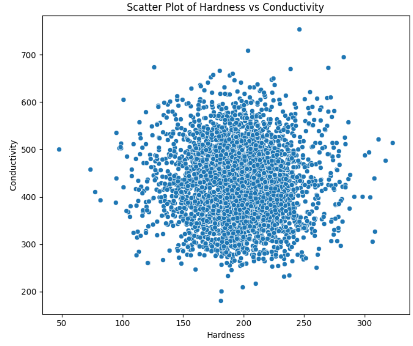
Yes, that’s exactly what you will see: a mess of dot plots. It’s not the fault of the scatter plot, as it is designed to place a dot for each data point in the dataset. While it is still a good and effective approach to see the relationship between two variables, in this case, it is really not helpful.

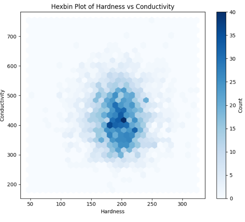
So let’s give hexbins a chance to make this data a bit more beautiful! Unlike scatter plots, which display individual data points, a hexbin plot uses a color gradient to represent the density of data points in each hexagonal bin. This means that instead of showing individual dots, it colours the hexagons to indicate where the density of data points is higher, making it easier to identify patterns and trends in large datasets.

It’s cool, right? It definitely enhances the readability of the chart. But we’re not finished yet! Let’s further improve our graph to make it even more useful. Suppose we have a dataset with latitude and longitude coordinates for house prices. We can use hexbins to display the median house value at specific locations on a map. This approach significantly improves readability, as the data points will be represented with a gradient instead of numerous individual dots.

Hexbins in Python

Now that we have a basic understanding of hexbins, it’s time to visualize a dataset. In this article, we will use the California Housing Prices dataset, which provides the latitude and longitude of median house value in California, making it very suitable for hexbins.

import pandas as pd
import seaborn as sns
import matplotlib.pyplot as plt

df = pd.read_csv("housing.csv")
df = df[["longitude" , "latitude" , "median_house_value"]]

Now we have a DataFrame that we imported from the housing.csv file, and we split the dataset into three columns. Now we are ready to create a plot. First, we will try a scatter plot to visualize density of prices in California.

plt.figure(figsize=(12, 8))
scatter = sns.scatterplot(data=df, 
                          x="longitude", 
                          y="latitude", 
                          hue="median_house_value",          
                          palette=sns.color_palette("RdYlGn_r", as_cmap=True),  
                          size=None,  
                          alpha=0.7,          
                          edgecolor=None)      

plt.title("Median House Prices in California", fontsize=14)
plt.xlabel("Longitude", fontsize=11)
plt.ylabel("Latitude", fontsize=11)

plt.legend(title="Median House Value", bbox_to_anchor=(1.05, 1), loc='upper left')
plt.show()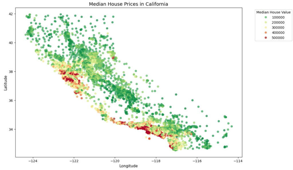

We can see the California map now, but it looks messy, making it difficult to determine whether prices are really high or low in specific locations. So, let’s change our method from a scatter plot to a hexbin plot and see how readability improves in our graph.

plt.figure(figsize=(12, 8))
hb = plt.hexbin(df['longitude'], df['latitude'], 
                 C=df['median_house_value'], 
                 gridsize=30, 
                 cmap='RdYlGn_r')

cb = plt.colorbar(hb)
cb.set_label('Median House Value')

plt.title("Median House Prices in California", fontsize=14)
plt.xlabel("Longitude", fontsize=11)
plt.ylabel("Latitude", fontsize=11)

plt.show()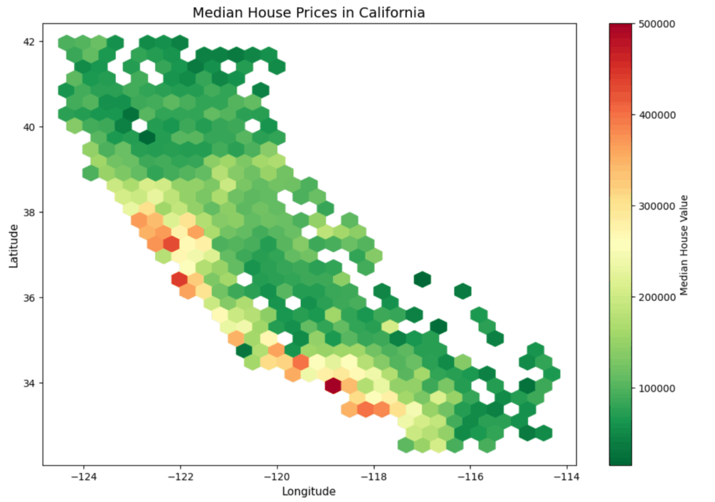

Hexagons are much easier to read than individual dots, allowing us to clearly see price changes on the map. As expected, we can also observe that house prices on the sides are higher than in other areas.

Conclusion

Hexbins may be less common than scatter plots, but they are particularly useful for large datasets where data points are densely clustered in specific areas. In such cases, scatter plots can become cluttered, making it difficult to identify patterns and trends. Hexbin plots aggregate data into hexagonal bins, providing a clearer visualization of data density and distribution.

This approach enables us to easily see variations in values through color gradients, helping us identify areas of high and low prices more effectively. Our analysis of house prices in California demonstrates how hexbins enhance readability and reveal insights that scatter plots might obscure. Overall, while scatter plots excel at displaying individual data points, hexbins provide a powerful alternative for summarizing and visualizing large datasets.